
Figure: A footbal fan excited for his team. Image generated by an AI model.
Suppose a new striker joins your favorite Bundesliga team. Fans are excited, the club has paid an enormous transfer fee, and expectations are huge. The new season starts. And then, he only scores a single goal in his first ten games. As a football fan of the impatient kind, you may be quick to lose faith in your new signing. But isn't that a bit premature after just ten games? Did the new striker maybe just have a few unlucky matches? And should you really be shouting at the TV?
Let’s take a step back. Indeed, if the striker’s lack of success continues, the Law of Large Numbers 1 tells us that, eventually, your concerns will be justified (perhaps not the shouting though). The Law of Large Numbers states that as the number of trials in a random experiment increases, the average of the results will get closer to the expected value. The empirically observed average number of goals per game will approach the true expected number of goals per game, provided each of his performances is an independent sample from some underlying distribution. Formally, if we denote \( Z_1, \dots, Z_n \) for the number of goals scored in each of the first \( n \) games, then the average number of goals \( \hat{\mu} = \frac{1}{n} \sum_{i=1}^n Z_i \) will converge to the number of expected goals \( \mu = E[Z_1] \) as \( n \) goes to infinity (under some mild assumptions).
This convergence can be made quantitative using what is called Hoeffding’s inequality 2. Assuming for the moment that scoring more than ten goals will almost never happen, the probability of your estimate \( \hat{\mu} \) deviating from \( \mu \) by more than some small \( t > 0 \) can be bounded by
$$
P(| \hat \mu_n - \mu| > t) \le 2\exp(-nt^2/50)
$$
This result can be seen as a quantitative version of the Law of Large Numbers: Note that as the number of observations \( n \) grows, the probability of over- or underestimating the population mean \( \mu \) by more than a fixed budget of \( t \) decays to zero. Importantly, you do not need any assumptions on the parametric form of the distribution for this to be true.
From Estimation to Prediction
So far, so good. We now know how long we can stay calm before we angrily sell the new striker. But as machine learning enthusiasts, we are naturally not content with just estimating means. Wouldn't it be far more interesting to predict whether a player will score based on a bunch of features \( x \) you have collected before the game (strength of opponent, his recent form, home or away)?
Denoting \( x \) for these features and \( y \) for the binary label (whether or not the player scores), let us find a model \( h \) that predicts \( y \) from \( x \). For example, \( h \) could be a logistic regression, or a decision tree. Once fitted, you can assess the model's quality using a loss \( l(y, h(x)) \) that is zero if your prediction is correct, and one otherwise. Ideally, you want to find a good \( h \) such that this loss is low on average: You are aiming to minimize
$$
L(h) = E_{x,y}[l(y,h(x))]
$$
which is called the risk of the predictor \( h \).
Since you do not have knowledge of the true underlying distribution \( (x, y) \), the best you can do is fit a model \( \hat{h} \) on a training dataset of \( n \) observations \( (x_1, y_1), \dots, (x_n, y_n) \), with each pair denoting an instance of features and labels. On this training data, you observe an empirical risk
$$
\hat L(\hat h) = \frac{1}{n} \sum_{i=1}^n l(y_i, \hat h(x_i))
$$
that evaluates how good \( \hat{h} \) performs on the training data. But is \( \hat{L}(\hat{h}) \) a reliable estimate of \( L(\hat{h}) \)?
If we want to trust our model to perform similarly when confronted with new data, we need the difference between \( \hat{L}(\hat{h}) \) and \( L(\hat{h}) \) to be small. You may be tempted to appeal to the Law of Large Numbers again, or call upon its quantitative cousin Hoeffding’s inequality. After all, isn’t \( \hat{L}( \hat{h}) \) just an empirical average that will converge to its population version \( L(\hat{h}) \) as the number of samples grows?
Uniform Laws of Large Numbers
Unfortunately, this does not work. The function \( \hat{h} \) that you fit on your training data explicitly depends on the observations \( (x_i, y_i) \). After all, \( \hat{h} \) is chosen precisely because it performs well on these observations. Therefore, the ordinary Law of Large Numbers does not apply.
This is where statistical learning theory comes in to the rescue. Instead of bounding the difference for the random predictor \( \hat{h} \), we look at the worst case difference between empirical and true risk over all possible predictors. Formally,
$$
\left| L( \hat h) - \hat L( \hat h) \right| \le \sup_{h \in H} \left| L(h) - \hat L (h) \right|
$$
While this may seem overly pessimistic at first, this simplification is the key to obtain useful bounds on \( L(\hat{h}) \). For example, suppose \( H \) only contains \( M \) predictors to choose from. Then, it can be shown that
$$
P \left( \sup_{h \in H} \left| L(h) - \hat L (h) \right| > t \right) \le 2M \exp(-2n t^2)
$$
which ensures that our model \( \hat{h} \) will not perform much worse on new, unseen data provided the sample size \( n \) is large. You will notice the similarity to the inequality we obtained earlier. However, the size \( M \) of the predictor class now also shows up on the right side, increasing the probability of underestimating the true risk of your model. In particular, when \( M \) is exponential in \( n \), you do not get a useful bound on \( L(\hat{h}) \).
Controlling Complexity
To make matters worse, \( M \) is rarely finite in machine learning—we typically optimize over function spaces with infinitely many possible predictors in them. Fortunately, statistical learning theory sometimes allows us to replace \( M \) with finite quantities that essentially capture the complexity of the predictors in \( H \).
Two standard tools to measure this complexity are the VC dimension 3, which essentially tells us how many binary patterns models from \( H \) can fit, or Rademacher complexity, which measures the capacity of \( H \) to fit random noise. For both, the intuition is the same: The more wild the predictors from \( H \) potentially behave, the less you can trust the empirical risk to be an accurate estimate of the true risk. Then again, keep in mind that a certain level of complexity in \( H \) is unavoidable if you want a good model.
With these tools, it becomes possible to bound the risk for large classes of predictors, including linear models, decision trees, or support vector machines.
Outlook
Admittedly, this is a bit of a classic view on things. In today’s world, we train models with billions of parameters that can in fact fit any function you want, making standard bounds on \( |L(\hat{h}) - \hat{L}(\hat{h})| \) vacuous. It remains one of the mysteries of deep learning why it still produces models \( \hat{h} \) that generalize well. Broadly speaking, it is believed that the architectures and optimization schemes used in deep learning guide the model to "nice" solutions, but the question is far from resolved.
Then again, not every powerful function class is as much of a mystery as are deep neural networks: For kernel machines, it is a lot easier (though still challenging) to precisely characterize the risk of the learned predictors. Since some neural networks actually behave like kernel models 4, these insights can be used to say something about neural networks after all. But that's a story for another day—perhaps the next half time break.
References
1.Klenke, Achim. Probability theory: a comprehensive course (Chapter 5). Springer Science & Business Media, 2013.
2.Vapnik, Vladimir N. "An overview of statistical learning theory." IEEE transactions on neural networks 10.5 (1999): 988-999.
3.Jacot, Arthur, Franck Gabriel, and Clément Hongler. "Neural tangent kernel: Convergence and generalization in neural networks." Advances in neural information processing systems 31 (2018).
4.Jacot, Arthur, Franck Gabriel, and Clément Hongler. "Neural tangent kernel: Convergence and generalization in neural networks." Advances in neural information processing systems 31 (2018).