
Figure 1: Schematic illustration of different strictly proper scoring rules that admit the same unique minimum but correspond to a different decision geometry (Image generated using ChatGPT 5.5).
How do we judge whether a probabilistic prediction is any good? When a forecast comes with a full distribution over possible outcomes rather than a single number, we need a principled way to score it against what actually happened. Proper scoring rules provide exactly this: a class of scoring functions designed so that a forecaster or predictive model can only minimize their expected score by reporting their true beliefs. This article introduces the basic idea, presents the most commonly used examples, and shows how the same concept connects classical statistical estimation with modern machine learning, where proper scoring rules are increasingly used to train neural networks and to quantify predictive uncertainty.
Proper scoring rules and decision geometry
Imagine forecasting tomorrow's temperature y ∈ ℝ. Rather than committing to a single number, a probabilistic forecaster issues an entire distribution P over possible outcomes. Consider two different prediction strategies: The climatological forecaster always reports the long-run distribution of temperatures for that day of the year, ignoring any current information; it is rarely wrong in a gross sense, but also never sharp. An informed forecaster, by contrast, uses today's atmospheric state to issue a much narrower distribution centered near the true outcome. Now, how can we assess which forecasting strategy is superior? A scoring rule S(P,y) assigns a numerical penalty to the forecast P once the observation y is revealed, rewarding predictions that are both sharp (concentrated) and well-located (centered near y). Crucially, we want such a rule to be proper: the informed forecaster should never be able to improve its expected score by misreporting its true predictive distribution, and the climatological forecaster should do best precisely when no further information is available. Let's formalize these ideas further:
Consider a general sample space 𝒴 and a convex class of probability measures 𝒫 over it. A scoring rule is a function S: 𝒫 × 𝒴 → ℝ such that, for every P ∈ 𝒫, S(P, ·) is a 𝒫-integrable function. The quantity S(P,y) denotes the score assigned to a forecast (or probabilistic prediction) P ∈ 𝒫 and a subsequent observation y ∈ 𝒴. Intuitively, a scoring rule measures how well the predicted P matched the outcome y, with a lower score indicating a better prediction. We define
$$S(P,Q) = \mathbb{E}_{Y \sim Q} [S(P,Y)], \quad P,Q \in \mathcal{P}$$
for the expected score of P under Q. The scoring rule S is called proper relative to 𝒫 if
$$S(Q,Q) \leq S(P,Q), \quad \text{for all }\ P,Q \in \mathcal{P}$$
It is called strictly proper (relative to 𝒫) if equality holds if and only if P = Q[1]. The propriety condition has a simple interpretation: if the outcomes are truly generated by Q, then no forecast scores better in expectation than Q itself. In other words, a proper scoring rule rewards honest forecasting; there is no incentive to report anything other than one's genuine belief about the distribution of the outcome.
Every scoring rule S can be associated with a corresponding (generalized) entropy and (generalized) divergence, which are defined for P,Q ∈ 𝒫 as
$$H(P) = S(P,P)$$
$$D(P,Q) = S(P,Q) - H(Q)$$
The entropy H is strictly concave on 𝒫 and can be thought of as a measure of how much uncertainty is inherent in the distribution P. The divergence D is a pre-metric and essentially measures the distance between two probability measures P and Q.
In the following we give important examples of commonly used (proper) scoring rules, focusing on the case of a univariate real-valued sample space. In particular, consider a (measurable) sample space 𝒴 ⊆ ℝ and a probabilistic prediction P ∈ 𝒫 with corresponding Lebesgue density p.
Logarithmic score
The logarithmic score (LogS), defined by
$$\mathrm{LogS}(p,y) = - \log p(y)$$
is strictly proper relative to the class of probability measures that are absolutely continuous. Its entropy and divergence are given by the well-known Shannon entropy
$$H(P) = - \int p(x) \log p(x) \, d \mu(x)$$
and Kullback–Leibler divergence
$$D(P,Q) = \int q(y) \log (q(y) / p(y)) \, d \mu(y)$$
Quadratic score
The quadratic score (QS), defined by
$$\mathrm{QS}(p,y) = |p |_2^2 - 2p(y)$$
is strictly proper relative to the class of probability measures with finite second moment. Its entropy is given by H(P) = ‖p‖² and its divergence by D(P,Q) = ‖p − q‖², where p,q denote the densities of P,Q ∈ 𝒫.
Continuously ranked probability score
The continuous ranked probability score (CRPS), defined by
$$\mathrm{CRPS}(P,y) = \mathbb{E}_{Y \sim P} |Y-y| - \frac{1}{2} \mathbb{E}_{Y,Y' \sim P} |Y-Y'|$$
is proper with respect to all probability measures on ℝ and strictly proper relative to the class of probability measures with finite first moment. The CRPS admits the entropy H(P) = ½ 𝔼Y,Y′∼P|Y−Y′| and the (symmetric) divergence
$$D(P,Q) = \int (F_P(y) - F_Q(y))^2 \, dy$$
with FP (FQ) denoting the cumulative distribution function of P (Q).
It is evident that different scoring rules not only assign a different score between a predicted distribution P and a true observation y, but also lead to a completely different decision geometry on the space of probability measures 𝒫, induced by the corresponding entropy and divergence functions. The downside of this flexibility is that no single scoring rule is universally best: the appropriate choice depends on the task, and proper scoring rules can differ substantially in computational cost and in how they scale to high-dimensional predictions. In the following figure, the difference in scores is highlighted for a predictive Gaussian distribution.

Figure 2: Comparison of different scoring rules and their corresponding values for different predictive Gaussian distributions and realized outcomes y. The logarithmic score behaves quadratically in y, while the CRPS behaves quadratically only locally and linearly for large values of y. The quadratic score is nonconvex and bounded from above. Thus all three scoring rules impose a different penalty on the predictive distribution with respect to a realization y from the true distribution.
The statistical side of things
Scoring rules can be used for statistical parameter inference by making use of so-called M-estimators[2]. In particular, let Θ ⊆ ℝp denote a space of parameters and {Pθ, θ ∈ Θ} a corresponding parametric family of distributions for Y ∈ 𝒴. A typical example would be the normal distribution {𝒩(·; μ, σ²), (μ, σ²)ᵀ ∈ Θ ⊆ ℝ × ℝ₊}.
Further, consider a random sample (y1, …, yn) from Pθ and denote by P̂ the empirical distribution of the sample. Then, given some strictly proper scoring rule S, an estimate of θ can be obtained via
$$\hat{\theta}_S = \arg\min_\theta \sum_{i=1}^n S(P_\theta, y_i)$$
The above is called the minimum score estimator of θ[3]. Importantly, one can show that for any proper scoring rule and any family of distributions, under some regularity conditions on the model, the estimator is asymptotically normally distributed as
$$\hat{\theta}_S \approx \mathcal{N}(\theta, (nG(\theta))^{-1})$$
Here, G(θ) denotes the so-called Godambe information matrix[3]. This asymptotic normality can be used to derive confidence intervals or p-values for statistical hypothesis tests.
Note that in the special case of the logarithmic score, one recovers the classical maximum likelihood estimator, for which the Godambe information matrix collapses to the inverse Fisher matrix, and the resulting estimator is asymptotically efficient, attaining the Cramér–Rao lower bound in the limit[4]. However, this only holds if the true model lies within the specified family {Pθ, θ ∈ Θ}. In general, this cannot be expected, especially in complex learning settings such as those arising in machine learning. When the model is misspecified, the estimate depends heavily on the selected scoring rule, and using, for example, the CRPS can offer robustness advantages beyond the logarithmic score.

Figure 3: Estimated densities p̂(y) for different scoring rules obtained via minimum score estimation, where the assumed model is a Gaussian and the true model follows a Student-t distribution. In the limiting case ν → ∞, where the Student-t is approximately Gaussian, all three estimators recover the true parameter and density. For small ν, the logarithmic score leads to a poor fit, while the quadratic score and CRPS estimates yield a density that is more similar to the underlying true density. This highlights the robustness of different scoring rules with respect to model misspecification. In particular, the quadratic score and CRPS are less sensitive to outliers.
The machine learning side of things
Recently, proper scoring rules have been successfully combined with neural network training to improve performance in predictive modeling. On the one hand, neural networks can be specified to predict a (conditional) parametric distribution Pθ, which is then optimized using minimum score estimation. Here, scoring rules such as the CRPS have shown great success, due to their robustness to model misspecification and their tendency to provide calibrated predictions. Model misspecification describes the typical case where no candidate model perfectly captures the underlying data distribution, whereas calibration means the forecasts are trustworthy in a probabilistic sense, for instance, outcomes predicted with 80% confidence should materialize about 80% of the time. This has been applied to problems such as parameter inference[5], forecasting[6], and weather post-processing[7],[8].
More generally, scoring rules such as the CRPS do not require an underlying probability density and can be computed from samples alone. This makes it possible to train neural networks by injecting random noise and optimizing a suitable proper scoring rule, thereby approximating any (conditional) nonparametric distribution. This method has shown state-of-the-art performance in regression benchmarks[9], while also providing extrapolation guarantees[10]. Furthermore, the approach has been extended to other domains, yielding leading predictive models in dynamical systems[11] and especially weather forecasting[12],[13],[14].
Finally, recent work has focused on using proper scoring rules to construct uncertainty measures that quantify how certain a predictive model is about the predictions it issues[15],[16]. In particular, the entropy and divergence functions associated with a scoring rule act as natural measures for aleatoric (irreducible) and epistemic (reducible) uncertainty, respectively. This construction includes the already well-known uncertainty measures based on entropy, i.e. the logarithmic score. However, extending it to other scoring rules allows for a more robust assessment of uncertainty and improved performance in downstream tasks[16].
Conclusion
In summary, proper scoring rules offer a principled framework for evaluating probabilistic predictions, rewarding forecasters for reporting their true beliefs while inducing a rich geometry on the space of probability measures through their associated entropy and divergence functions. The choice of scoring rule matters in practice: it shapes the robustness of statistical estimation under model misspecification and underpins a growing range of machine learning methods, from training probabilistic neural networks to quantifying predictive uncertainty.
References
[1] Gneiting, T. and Raftery, A. E. (2007). Strictly Proper Scoring Rules, Prediction, and Estimation. Journal of the American Statistical Association 102, no. 477 (2007): 359–78. ↩
[2] Huber, P. J. and Ronchetti, E. M. (2009). Robust Statistics. John Wiley and Sons, New York. ↩
[3] Dawid, A. Philip, and Musio, M. (2014). Theory and Applications of Proper Scoring Rules. METRON 72, no. 2 (2014): 169–83. ↩
[4] Vaart AW van der. Asymptotic Statistics. Cambridge University Press; 1998. ↩
[5] Pacchiardi, L. and Dutta, R. (2022). Likelihood-Free Inference with Generative Neural Networks via Scoring Rule Minimization. arXiv:2205.15784. ↩
[6] Pacchiardi, L., Adewoyin, R. A., and Dueben, P. (2024). Probabilistic Forecasting with Generative Networks via Scoring Rule Minimization. Journal of Machine Learning Research, 25(45):1−64. ↩
[7] Rasp, S., and Lerch, S. (2018). Neural Networks for Postprocessing Ensemble Weather Forecasts. Mon. Wea. Rev., 146, 3885–3900. ↩
[8] Schulz, B., and Lerch, S. (2022). Machine Learning Methods for Postprocessing Ensemble Forecasts of Wind Gusts: A Systematic Comparison. Mon. Wea. Rev., 150, 235–257. ↩
[9] Kelen, D., M., Jung, A., Kersch, P., and Benczur, A. A. (2025). Distribution-Free Data Uncertainty for Neural Network Regression. Thirteenth International Conference on Learning Representations. ↩
[10] Shen, X., and Meinshausen, N. (2025). Engression: extrapolation through the lens of distributional regression. Journal of the Royal Statistical Society Series B: Statistical Methodology, Volume 87, Issue 3, Pages 653–677. ↩
[11] Bülte, C., Scholl, P., and Kutyniok, G. (2025). Probabilistic neural operators for functional uncertainty quantification. Transactions on Machine Learning Research. ↩
[12] Lang, S., Alexe, M., Clare, M.C.A. et al. (2026). AIFS-CRPS: ensemble forecasting using a model trained with a loss function based on the continuous ranked probability score. npj Artif. Intell. 2. ↩
[13] Alet, F. et al. (2025). Skillful joint probabilistic weather forecasting from marginals. arXiv:2506.10772. ↩
[14] Bonev, B. et al. (2025). FourCastNet 3: A geometric approach to probabilistic machine-learning weather forecasting at scale. arXiv:2507.12144. ↩
[15] Kotelevskii, N., Kondratyev, V., Takáč, M., Moulines, E., and Panov M. (2025). From Risk to Uncertainty: Generating Predictive Uncertainty Measures via Bayesian Estimation. Thirteenth International Conference on Learning Representations. ↩
[16] Bülte, C., Sale, Y., and Kutyniok, G. (2025). Uncertainty Quantification for Regression: A Unified Framework based on kernel scores. arXiv:2510.25599. ↩
About the Author
Christopher Bülte, MSc is a doctoral researcher specializing in the intersection of neural networks, uncertainty quantification and physical systems at Prof. Gitta Kutyniok's Chair for Mathematical Foundations of Artificial Intelligence at LMU Munich. As a member of relAI, his research focuses on developing novel probabilistic and uncertainty quantification-related methods for neural networks with applications in meteorology, dynamical systems, energy systems or quantum physics.