Quantifying Uncertainty of the Treatment Effects

Fig. 1. Pearl's ladder of causation. The treatment effect, , as a random variable, is situated on the third, counterfactual level of causation. Source: Melnychuk et al. 2024.

When we talk about understanding the effect of a medical treatment or policy intervention, we usually refer to the “average” effect: for instance, the average increase in a patient’s survival time or the average reduction in infection rates. However, in real-world decision-making, especially in safety-critical fields such as healthcare, it’s vital to go beyond averages and understand the uncertainty of individual responses. This post introduces ideas from a recent NeurIPS 2024 paper on quantifying the uncertainty of treatment effects (Melnychuk et al. 2024).

The identification and estimation of treatment effects is a challenging task for two main reasons:

1. The treatment effect is a counterfactual, non-observable random variable (see Fig. 1): We never observe what would have happened under a different treatment for the exact same individual. Crucially, that unobserved outcome remains counterfactual, creating additional uncertainty that can’t be fixed just by collecting more data: Even when this data is experimental (interventional) as in randomized control trials (RCTs).
2. In observational studies, we additionally do not have full control over the treatment assignment — people in the data “chose” or “were assigned” treatments in ways that might correlate with their characteristics. Those characteristics are known well under the term confounders, and their presence complicates any downstream estimation or machine learning.

This post examines key concepts from the new approach, how the authors addressed these challenges, and why these ideas matter.

A Quick Primer: Averages vs. Uncertainty

In many medical or policy-related studies, you’ll see the term CATE (Conditional Average Treatment Effect): , see (Curth et al. 2021). It represents how much a treatment in changes the outcome on average for individuals with specific characteristics (or covariates) . For instance, if the CATE for a particular demographic is +2 years to life expectancy, we might say “they benefit by about 2 years on average.”

But outcomes vary — they are not always pinned down to a single number. Even if two patients share similar covariates, one might react very differently from the other to the same treatment. This inherent randomness (sometimes called aleatoric or irreducible uncertainty) can be critical: if a cancer drug has a positive average effect but also a nontrivial chance of causing serious side effects, you want to know that risk before prescribing it.

Key problem: The distribution of the treatment effect itself — the difference between potential outcomes under treatment and under non-treatment — cannot be pinned down exactly from observational or even experimental data alone. We only see one version of the outcome for each individual, never the other potential outcome that didn’t happen.

In machine learning, we often separate “epistemic” from “aleatoric” uncertainty:

• Epistemic uncertainty: The uncertainty that comes from lack of knowledge — often reduced by getting more (or higher-quality) data or improving the model.
• Aleatoric uncertainty: The inherent randomness in the phenomenon; you can’t make it go away by gathering more data.

For treatment-effect problems, it’s not always enough to say, “On average, you’ll do well under this drug.” You want to know the chance that you won’t benefit—or even be harmed. That’s precisely what aleatoric uncertainty of the treatment effect addresses.

Makarov Bounds and Partial Identification: Why “Bounds” Instead of a Point Estimate?

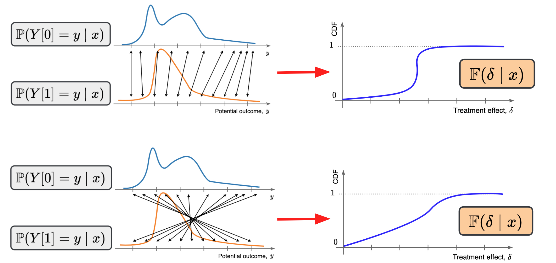
Fig. 2. Fixed distributions of potential outcomes yield two different distributions of the treatment effect (depending on how the counterfactual outcomes are coupled). Source: Melnychuk et al. 2024.

Because we can’t observe the counterfactual outcome, the true distribution of treatment effects (the full spread of possible gains or losses across individuals) is non-identifiable (see Fig. 2). For example, instead of yielding a specific value for some distributional aspect of the treatment effect (e.g., density or cumulative distribution function), we have a region of all plausible values consistent with our observational data.

In our work, we leverage so-called Makarov bounds. These bounds basically say: given the data you can see — such as the distribution of outcomes under treatment and the distribution of outcomes under non-treatment — what are the minimum and maximum probabilities that a person experiences a certain level of benefit (or harm) from the treatment? The result is an interval or band that captures all feasible treatment-effect distributions consistent with the observed outcomes.

This approach is an example of partial identification: instead of claiming “the treatment effect distribution is exactly this,” it says, “the treatment effect distribution must lie between these two extremes, given the available data and assumptions.”

The AU-Learner: A Novel Approach

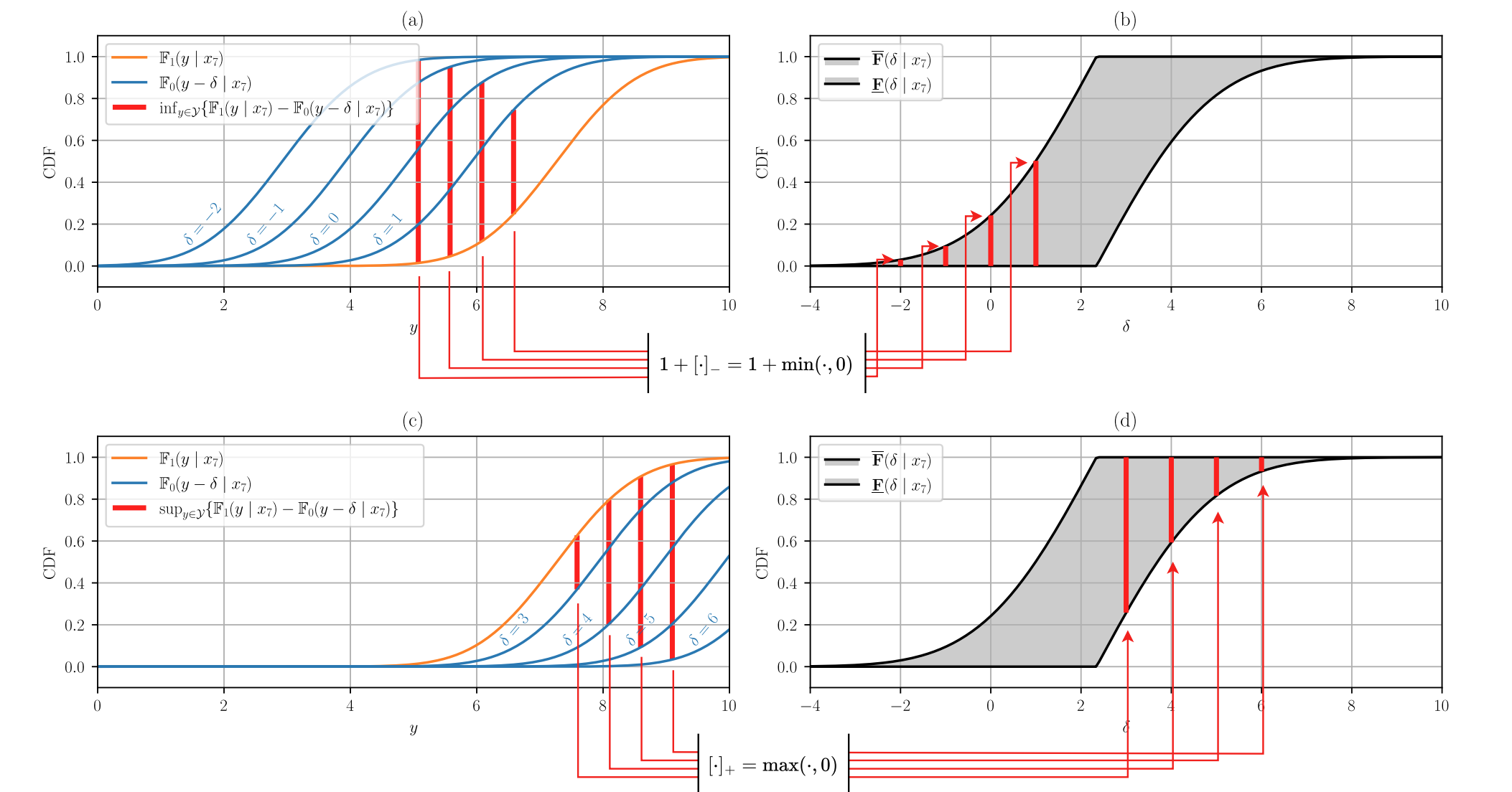
Fig. 3. Construction of the Makarov bounds of the cumulative distribution function of the treatment effect. Source: Melnychuk et al. 2024.

The NeurIPS 2024 paper (Melnychuk et al. 2024) introduces an AU-learner (short for “Aleatoric-Uncertainty Learner”) to estimate bounds on the distribution of the treatment effect. Some noteworthy points about this method:

1. Orthogonal Learning:
   It uses a concept known as Neyman-orthogonality, which makes the estimation process less sensitive to small mistakes in underlying nuisance functions (nuisance functions have to be used as we cannot learn the distribution of the treatment effect directly from data). Orthogonality effectively stabilizes the final estimate and increases the efficiency of the estimation/learning.

2. Flexible Neural Components:
   The method's instantiation is built on normalizing flows (a popular flexible model for probability distributions) to model the distributions for each potential outcome. By plugging these distributions into Makarov bounds, they produce upper and lower bounds for the treatment-effect distribution — conditioning on individuals’ covariates.

3. Partially Identified Inference:
   Because the distribution is not point-identifiable, the AU-learner yields a range of plausible scenarios. This is more honest than relying on additional identifiability assumptions: Our framework only assumes the regular potential outcomes framework assumptions.

Why It Matters (Especially in Medicine)

Imagine a scenario where a new treatment can drastically help many patients, but there’s a moderate chance of severe side effects that lead to worse outcomes. Policymakers or clinicians might want to see the fraction of people who will likely benefit versus the fraction who could be harmed. Traditional methods focusing only on averages might overlook that “substantial minority” who experience harm. By learning bounds on the entire distribution of gains and losses, we can inform safer, data-driven decisions.

References & Further Reading

• V. Melnychuk, et al. "Quantifying Aleatoric Uncertainty of the Treatment Effect: A Novel Orthogonal Learner". NeurIPS 2024. https://arxiv.org/abs/2411.03387
• A. Curth, et al. “Nonparametric Estimation of Heterogeneous Treatment Effects: From Theory to Learning Algorithms”. AISTATS 2021. https://arxiv.org/abs/2101.10943
• N. Kallus, “What’s the Harm? Sharp Bounds on the Fraction Negatively Affected by Treatment”. NeurIPS 2022. https://arxiv.org/abs/2205.10327

(This post is based on the NeurIPS 2024 paper titled “Quantifying Aleatoric Uncertainty of the Treatment Effect: A Novel Orthogonal Learner. The work was produced in the scope of a research stay at the University of Cambridge, funded by the Konrad Zuse School of Excellence in Reliable AI.)