Whenever we want to detect where certain structures are in an image -- we might want to detect roads in a satellite photo, a specific organ in a medical scan, or the foreground object in a picture we took on our phone -- we have a segmentation task at hand. One of the most natural ways to approach such a task is by training a neural network to segment the image: For each pixel in the image, the network should tell us whether this pixel belongs to the object we are looking for or not. Such a neural network is called a segmentation network.
The goal that segmentation networks are typically trained for is, roughly speaking, to get a large proportion of pixels correct. However, it can easily happen that such networks make topological errors: For example, two segments of road may end up disconnected, or the detected organ has an unexplainable hole in the middle. To illustrate this, let's have look at this output from a cell segmentation task:
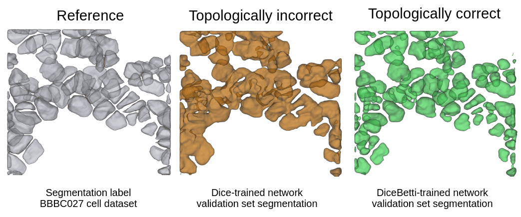
The left image is the true segmentation label. There are a number of distinct cells which are not connected, but the gaps that separate them are quite thin. The middle output is from a network trained with the Dice loss, which is one of the standard loss functions for training segmentation networks [1]: While cells are predicted in the correct location, they have mostly grown together to one big blob instead of being separated. Determining the number of cells from such an output would be very difficult.
The image on the right shows what we can achieve instead if we take topological properties into account during training. Cells are separated much better here. This is a little teaser to the topological loss function we'll discuss at the end of this blog post. But before we get to that, we need to discuss what we even mean with "topological properties".
Analyzing the topology of 2D images
In our context, analyzing the topology of a 2D image boils down to identifying two kinds of structures: connected components and holes. In 3D we can furthermore identify cavities (empty space that is fully enclosed, an "air pocket", so to say).
This needs an example: Let's analyze the topology of the relAI logo.

This should be fairly simple. Clearly, the image has two holes (in the "e" and the "A"), and a small number of connected components (I count 23). Right?
Unfortunately, the computer disagrees:
>>> import betti_matching
>>> # [..] load image: relai_logo_grayscale = ...
>>> result = betti_matching.compute_barcode(relai_logo_grayscale)
>>> print(f"{result.num_pairs[0]+1} connected components,"
...       f"{result.num_pairs[1]} holes")
4245 connected components, 1124 holes
That's a lot of connected components and holes! What's going on here, and where do these numbers come from?
The discrepancy comes from the fact that the algorithm reports topological features across all possible binarization thresholds. Topological features such as connected components or holes are per se defined only on binarized images (each pixel is either white - that is, empty space - or black - that is, filled space). Binarizing the image at a threshold  means that we make all pixels with a brightness higher than white, and all other pixels black. This is the relAI logo binarized at three different thresholds:

While the leftmost image has only five connected components, the other images have much more. We need to decide which threshold we want to use for the computation of topological features. We might be able to choose a good threshold for a clean image like this, but on more complicated images, picking one single threshold will usually not allow us to capture all topological structures we are interested in [2].
What we can do instead is to compute the topological features of the image across all possible binarization thresholds. Since a feature is usually "alive" at more than one threshold, we need to make sure that we do not count it more than once: For example, the hole in the letter "e" exists at the threshold  , and still exists at
  , even though the empty space it encloses has become a bit smaller as a few more filled pixels have been added. We want to consider both instances of the hole at the two different thresholds as the same hole. Luckily, it's possible to track a feature across a range of thresholds, while keeping track of the information that it's fundamentally the same feature.
The mathematical framework that allows us to do this is called persistent homology. Homology is the part that lets us formally define topological features, such as holes and connected components [3]. Persistence refers to taking the lifetimes of features into account (features with a long lifeftime persist over a wide range of thresholds). I will not go into the mathematical details here, but I'll put some pointers at the end of the post in case you are curious to learn more.
If we can track features across a range of thresholds, this furthermore means that we can track the lifetime of features -- the range of thresholds at which they exist. We will see shortly how this enables us to distinguish important features from unimportant ones.
Let's have a look at all the holes that we can find in the relAI logo at different thresholds. You can play around with this interactive demo and change the threshold value by dragging left/right to see which features come into existence or disappear.
Try the interactive demo on GitHub
In our example, there are many features with very short lifetimes: These are the features that come from noise. There are much less features with longer lifetimes: those are the relevant features, in this case the hole in the "e" and the "A". A long lifetime corresponds to a high contrast in the image, and taking this into account, we can tell apart the relevant features from the irrelevant ones. This explains the high number of features we saw in the Python snippet above: The persistent homology algorithm reported 4245 connected components and 1124 holes, but the bulk of them are short-lived features that are not visible to the naked eye.
We can assemble the lifetimes of all features into a persistence barcode: Each feature is represented by an half-open interval (or bar)  of its birth and death intensity values. In our example, the barcode describing the holes consists of a bar
  for the "A", a bar
  for the "e", and a lot of much shorter bars for the features that come from noise.
Persistent homology for segmentation loss functions
So, how does all of this relate to image segmentation? As I said in the beginning, your typical segmentation loss (e.g. the Dice loss) does not focus on topology in particular. It may not prevent topological errors from happening, especially if they are caused by a small number of incorrect pixels. However, one can construct a topological loss function using persistent homology, and even pass gradients through it such that it can be used for training.
When we use a segmentation network, the network outputs a likelihood value for each pixel, a value between 0 and 1 that represents how likely the network thinks this pixel is a part of the segmented object. This is convenient for us: instead of grayscale image intensity values, we can feed these likelihood values into a persistent homology computation. The idea is to compare the persistence barcode of the binary ground-truth label with the barcode of the predicted likelihood map, and try to make the two barcodes more similar during training. This was pioneered in Hu et al. 2019: Topology preserving Deep Image Segmenation, where a topological loss term would influence the prediction output to have the right number of topological features.
The idea was further developed in Stucki et al. 2023: Topologically Faithful Image Segmentation via Induced Matching of Persistence Barcodes by not only enforcing the correct number of topological features, but also matching spatially related topological features (via the Betti matching) to make sure that the right features would be reinforced or eliminated.
During training, the Betti matching loss function prescribes gradients for single pixels in the prediction: Each topological feature is born at a specific pixel and dies at another pixel, and the gradient descent algorithm pushes the intensities of these two pixels closer towards the birth/death intensities of the ground truth[^4]. Because only few pixels are directly affected, it makes sense to combine the topological loss with a standard Dice loss.
As it turns out, an obstacle is the computation time required to compute persistence barcodes -- even more so if you want to take 3D outputs into account. I worked on this in my master's thesis, and we are now publishing an optimized software library which I contributed to (this is the betti_matching library from the Python snippet above).
Topology-guided training: a toy example
To conclude this blogpost, let's have a look at the Betti matching loss in action. We take the relAI logo in grayscale, but destroy it's topology a bit by adding a few rectangles that connect/disconnect parts of the logo and break up the "e" cycle.
We now run a gradient-based optimization on this image. To keep things simple, we will not use a neural network, but directly modify the pixels of the input image as prescribed by the gradient of the Betti matching loss between the altered grayscale image we are optimizing, and a binarized label computed from the unaltered original image.

The training successfully separates the fused-together connected components, and connects up or eliminates superfluous components (in case you're wondering: diagonally connected pixels do not count as connected for our purposes). It also restores the destroyed "e" cycle. On the other hand, the topological loss alone has no chance to bring the image in the original state -- it only cares about the topology. This is why, for example, parts of the "e" are now in the connected component belonging to the "r".
For this reason, we need to combine the topological loss with a more convential Dice loss. While the topological loss only cares about the critical pixels that can correct the topology, the Dice loss cares too little about those critical pixels. By combining the two, we can have the best of both worlds.
If you're interested in using this method, stay tuned: We published the Betti-matching-3D library with python bindings, and are working on a publication, currently available as an arXiv preprint.
Some references if you're curious to learn more
If you're curious about persistent homology (you'll also often see the term Topological data analysis, or TDA, for the type of data analysis that uses persistent homology as its main tool), here are some references you can look at:
- A Short Course in Computational Geometry and Topology by H. Edelsbrunner (2014).
- Computational Topology for Data Analysis by T. K. Dey (2022).
These books work on simplicial complexes (which are suitable for point-cloud data), while this blogpost is based on cubical complexes (which are suitable for image data).
- A book which focuses on homology on cubical complexes is Computational Homology by T. Kaczynski et al. (2004).
- We also give a brief introduction to the cubical complex setting in our preprint which I mentioned above.
[1]: In case you're not familiar with neural network training: A loss function measures how good (or rather, how bad) a prediction is, and the training process tries to minimize the loss function (usually bring it close to zero) over the training data. Different loss functions express different training objectives and may emphasize different goals. There are many metrics for binary classification (which image segmentation is, on a pixel-wise level): The simplest one would be accuracy, which measures the proportion of correctly predicted pixels. The commonly used Dice score (also called  -score) avoids some problems of the accuracy metric when classes are imbalanced. Those metrics are close to one when the performance is good, so in a loss function, we would use
  , where
  is the respective metric.
[2]: Even in this simple example, JPEG compression artifacts and anti-aliasing mean that the background is not uniformly white, and the letters are not uniformly black.
[3]: In homology, each hole is described by an equivalence class of all cycles that go around that hole. Cycles that go around the same hole are called homologous.
[4]: A small but important detail: In the segmentation setting, the foreground is described by high (instead of low) intensity values -- we build up the images from high values to low values instead of the other way around as we did before (in technical terms, we use a superlevel filtration instead of a sublevel filtration). Hence ground-truth features get born at 1.0 and die at 0.0.